MSCNM

Deriving Formulae

-Shreya Doshi

What do you think a formula is? Think about it. Do you think it is something that has an equal to sign in it? Are all = sign mathematical items formulae? No?

Now here’s what a formula’s definition is: a mathematical relationship or rule expressed in symbols. This is just what it is using complex words. To simplify, it is a uniform way of finding an answer. So basically using a formula you can find the answer to anything, crazy isn’t it?

We need and use these formulae to make life simple for us, instead of we doing the whole process every time. We can just input certain things into specific formulae and get our answers. We use formulae everywhere in our life, we just don’t realize it. Our brain functions on formulae and logic. Only that way we carry out our actions to certain stimulations. So there you go, now you know we use formulae in everything. Math is famously known for its formulae simply because it has so many of them. Although, do you know how we got to them?

What is the Quadratic Formula? (Explained with 9 Surefire Examples!)

Now that’s a really important question, how do we get or make formulae?

Pretty tough isn’t it?

It takes decades and centuries of research and multiple extraordinary mathematicians for just one formula to be formed. So, that’s how difficult it is just to make one formula. Now think about it we have so many formulae. How much time and effort must’ve been put into it! Although do you ever wonder how they got to the formulae? What must they have done? That’s the difficult part and that’s why we derive formulae to get to the root of it and to understand it, cause isn’t it better to understand the formula properly and know how it works from the bottom rather than just by hearting it. So, that’s why we derive formulae and we should always understand them properly. For instance, here I am going to derive the quadratic formula for you:

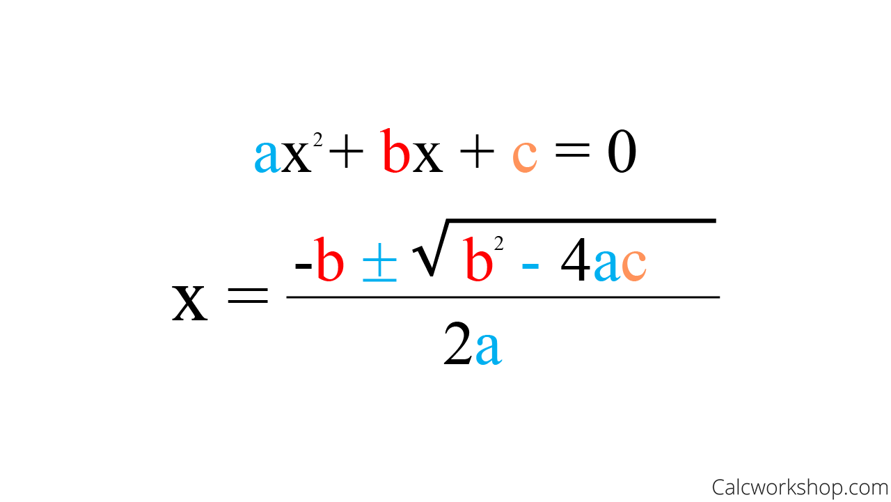
QUADRATIC FORMULA:

What is the quadratic formula?

Why do we use it? To find a solution of x, but from what? The quadratic equation.

What is the quadratic equation?

Now here let’s analyse the equation. There’s a common variable ‘x’ which we have to find and then there’s ‘a’, ‘b’ and ‘c’ as letters. Now what are these letters? These are nothing but the coefficients, otherwise known as numbers. We have used these letters a, b and c as we do not know these coefficient values and that’s the beauty of formulae. I can add any numbers instead of a, b and c and get my answer. All of this equates to 0 which makes it simple.

Next, the one thing you need to know is that the whole quadratic equation is centered and found by completing the square basically. So, what we now do, is complete the square and only then can we derive the formula as the formula is based on this.

First, to complete the square, the rule is that the coefficient to the squared term which is x2 should be 1. Now look up to the equation is it 1? No, it’s a, so now to remove this ‘a’ from there we have to divide the whole thing by ‘a’ such that we can nullify the ‘a’ on the x2 term. This is because as ‘a’ is in multiplication, we have to use division to remove it. So now the formula looks something like this:

Here there is no ‘a’ on x^2 as it is cancelled from both the numerator and denominator. And 0 divided by a will be 0.

Now we have to complete the square for ‘x’ so which all terms have ‘x’ in them? That’s right the first and second. We don’t need the ‘c’ term on the left hand side (LHS) so let’s move it to the right hand side (RHS) so that it looks like this:

This c term becomes negative because it was positive on the LHS so to bring it to the RHS, we have to switch signs.

Moving on, now comes the interesting part, the most important part: the part where you actually complete the square. Here, we have to complete the square of LHS. For that, there is a simple rule we can follow which is we half and square the term which has the variable with the power of 1 which would be this term:

Although while finding the last term, we do not have to use the variable as it is the first term-

Completing the square steps:

So now we half it and then we square it

1)Half it: (b/a)/2) so that would basically be (b/2a)

2)Square that now: (b/2a)^2

3) Add this to the LHS

Since we have added this new term, we cannot just leave it like that otherwise this whole thing will become imbalanced and will not work. So to balance it out we add the same thing on the RHS to nullify these. The whole equation looks like this:

Now observe the LHS carefully, do you see something cause I do. It’s a perfect square! That’s why we added the last term. And now since it’s a perfect square, we can simplify even further as we already know the identity. So as this is in an expanded form, we can compress it using identities.

That’s on the LHS, for the RHS we can easily expand the bracket and square that term.

So all in all this would look like:

Here we have simplified the LHS in the identity of (a+b)^2 = a^2 + 2ab + b^2. So we have simplified it backward.

Although why haven’t we taken (a-b)^2? This is because there is no negative sign in the LHS hence we use the first identity itself.

Now the RHS has two separate fractions which do not look that neat so how about we simplify them and make both they’re bases the same. For that we use LCM. As the c/a already has an a in the denominator, we can multiply that fraction by 4a such that both the denominators become 4a^2, although now even c will be multiplied with 4a. So this is how it’ll look:

Still looks a little messy right. But don’t worry we have completed stage one and we’re getting closer.

Next, since we have completed the square, now our aim is make x the subject as that is what the solution is.

The first step towards this is removing the square or the index and that is done by square rooting both the sides (LHS and RHS). here’s how it goes:

Now this is how the equation looks, although we can further simplify the RHS’s denominator so let’s do that so that the root is only of the numerators. This is how the RHS looks like:

Now it’s looking somewhat like it isnt it that’s cause we’re very close. Now we have to make x the subject hence we have to make the LHS only with x and move everything else to the RHS and since the 2 fractions have the same denominator, we can simply bring them together under one fraction to form what? You guessed it! The quadratic formula:

There you go! You have derived the quadratic formula. It wasn’t difficult right. And now you understand this better as well.

These quadratics have so many applications and uses and are so important to us as we need to use it in so many places. So now since you have a strong understanding of it, you can use this properly and be right about it instead of guessing it and hoping you are correct

This is just one of many formulae to exist, but now since you derived this, it is much better right? Now you should always try to derive and understand the why behind things and get to know where it all starts. Only then you can use the formulae properly. This shouldn’t only be for formulae but in fact for anything you learn instead of just by hearting it and remembering it for a couple weeks, understand the concept and remember it for the rest of your life.

REFRENCES:

https://www.chilimath.com/lessons/intermediate-algebra/derive-quadratic-formula/

https://www.onlinemathlearning.com/derive-quadratic-formula.html

Ramanujan Summation

-Nishant Oswal

I am sure you must have heard about various kinds of series during your high school. Remembering the formulae for their summation without knowing what practical application could such series have was boring, right? Not anymore. There are various interesting sequences which have surprising results. They have been used by researchers and scholars to develop various theories. One such among them is the ‘Ramanujan Summation’.

The results of the summation are so astonishing that it makes us question what we have been taught. For instance, if we have to find the sum of the first 50 natural numbers i.e. 1 + 2 + 3 + … + 50, we would use formula for the sum of n numbers of an arithmetic progression or directly the formula for the sum of first n natural numbers i.e. n(n+1)/2 So, we would get 50 * (51/2) = 1275 Now, what if we have to find the sum of all the natural numbers till infinity? Would it be a finite number? Would it be a positive number? You might think it would certainly be a positive number and probably the answer would also be infinity . But unfortunately, that is wrong. Can you believe the answer to the question is not a positive number? No, right? However, the summation results in -1/12 .

Srinivasa Ramanujan, who we today call ‘The Man Who Knew Infinity’, was among the first to give this summation and hence the name. Ramanujan was a natural genius. Ramanujan Summation essentially is a property of partial sums. The above summation also involves Euler-Maclaurin summation formula together with the correction rule using Bernoulli numbers.

Wondering how we got a rational number, let alone being negative?

Let us try to understand the proof of the above sum. However, it must be noted that the infinity that we talk about in this article is a countable infinite set, which is slightly different from the normal infinity that we know. The assumption is taken because only then would we be able to apply the mathematical properties.

We need to find,

Let us take,

What would result in? Either 0 or 1, right? Again, wrong. This series is divergent, a series where the infinite sequence of the partial sums of series do not have a finite limit. This type of divergent series is called Grandi’s divergent series. An interesting fact to note here is that, the result to this series of X can also be found using the geometric series i.e. the sum of infinite numbers of a Geometric Progression, only after making certain adjustments.

Coming back,

It seems like we are forcefully trying to arrive at the result of X = 1/2, but it is indeed true. The method we have used to get the value of X is not absolutely correct. We have to know much complex concepts like that of the Zeta Function to understand the same. For now, we take it to be 1/2

Now, let us consider,

Now, we have two equations,

It seems like some kind of magic. Doesn’t it? Well, that is the beauty of Mathematics. For years, this summation was highly debated. However, the result has been used in various theories of Physics. It has been used to derive equations in supersymmetric string theory. It was helpful in other areas of general Physics like to find the solution to the Casimir Effect, an effect arising from quantum theory of electromagnetic radiation.

One more interesting fact is that Ramanujan not only defined the sum of infinite natural numbers but he also defined the sum of the square of the infinite natural numbers and the sum of the cubes of infinite natural numbers i.e. 1^2 + 2^2 + 3^2 + … and 1^3 + 2^3 + 3^3 +4^3 + …

By now, you might have assumed that the answer to these series is also going to be something weird. Yes, you are right. The above sums result in 0 and 1/120respectively.

That is,

The above two sums can be proved using Riemann Integrals of real valued functions and hence it requires a deep knowledge about when the integral can be used.

At first, it might seem that Ramanujan’s work does not seem logical, and this is what mathematicians back then thought and hence neglected his work. However, after a few years, mathematicians got to know how the sums have been arrived at and it seems that he tried to convey something much deeper than what we know. Ramanujan would always be remembered for his great work and his contribution despite facing hardships and not having formal knowledge of advanced mathematics.

We will try to cover the proof of the remaining two summations in upcoming blogs after talking about Riemann Integrals. I hope you found this one insightful!

REFERENCES

https://www.iitk.ac.in/ime/MBA_IITK/avantgarde/?p=1417 ,

http://sersc.org/journals/index.php/IJAST/article/view/15653/7906 ,

https://www.hindupost.in/science-technology/the-ramanujan-summation-1-2-3-%E2%8B%AF-%E2%88%9E-1-12/ ,

https://inquiscitive.wordpress.com/2019/10/13/ramanujan-summation-is-it-an-overrated-mistake/ ,

https://en.wikipedia.org/wiki/Riemann_zeta_function .

The Math Behind Backgammon

-Sanskruti Mehta

We have all heard of the game Backgammon, right? Not many of us play it. For me, Backgammon was that confusing and old age game that was on the other side of my Chess board like a “Buy one, Get one free”. It is only now I know that Backgammon is quite interesting and was and is still a popular game. But did you know that you can raise your chances of winning by using a little Math? Turns out- there is Math behind backgammon.

How is it Played?

The image below shows how the backgammon board is setup in the beginning of the game.

The triangles seen are known as pips or points and the playing pieces are known as checkers or chips.

The points are numbered from 1 to 24. In the commonly used setup, each player begins with fifteen chips, two are placed on their 24-point, three on their 8-point, and five each on their 13-point and their 6-point. The two players move their chips in opposing directions, from the 24-point towards the 1-point. Points 1 through 6 are called the home board or inner board, and points 7 through 12 are called the outer board.

The objective is for players to remove (bear off) all their checkers from the board before their opponent can do the same.

To start the game, each player rolls one die, and the player with the higher number moves first using the numbers shown on both dice. In the course of a move, a checker may land on any point that is unoccupied or is occupied by one or more of the player’s own checkers. It may also land on a point occupied by exactly one opposing checker, or “blot”. In this case, the blot has been “hit”, and is placed in the middle of the board on the bar that divides the two sides of the playing surface. A checker may never land on a point occupied by two or more opposing checkers; thus, no point is ever occupied by checkers from both players simultaneously. There is no limit to the number of checkers that can occupy a point at any given time. Checkers placed on the bar must re-enter the game through the opponent’s home board before any other move can be made. When all of a player’s checkers are in that player’s home board, that player may start removing them; this is called “bearing off”.

The Math:

Now that we have understood how to play Backgammon, let us get to the main topic. As I revealed earlier, Backgammon is played often to win money. A doubling cube is used for this purpose. It is like poker in that sense. There is a big role of luck in the game. However, there are certain calculations that you can do to estimate how fast you can win and whether you have a chance to win: –

1) Pip Counting

Determining your position in this race is achieved by calculating the difference between the number of pips that you need to get all your checkers home and off the board, and the number our opponent needs. The technique is known as pip counting.

The pip count= the no of the point/pip x the no of checkers on that point/pip

The pip count is 167 for each player at the start of the game. This can be better understood with the help of an example.

In this example at the closing stage of a game, Red has two checkers on the 6 point and White has one checker on his 6 point and two checkers on his 2 point. Red requires 12 pips to completely bear off (6 × 2 = 12), while White requires 10 pips (6 × 1) + (2 × 2) = 10. Therefore, the pip count informs us that Red is 2 pips behind in the race.

The pip count is an essential factor in many cube decisions and can help in determining the appropriate choice of strategy while playing.

2) Probability

While you cannot predict what will be the 2 numbers that come face up on your dice, you at least can know the probability of a certain number or numbers turning up face up. Since each die has 6 numbers the number of possibilities or the summation of the sample space is 36. This can draw many probabilities.

For example, the probability of a double coming up (same number on both dies) is 6/36 or 1/6. Now how can you use your probability skills to improve your strategy?

Let’s say, that this is how your board looks like. This reveals that one of the most dangerous points on which to leave a blot is 7. Twenty-four dice permutations can hit a blot exposed on that point. To a beginner it looks almost suicidal to move onto 7 with an opening move, 66% chance that your opponent will hit you. Yet many of the most expert players use this as an opening move. If you do this there are:

19 chances in 36 that he can hit you but is forced to leave a blot.
12 chances in 36 that he will miss your blot.
5 chances in 36 that he can hit you and cover his blot. (i.e. 6:6, 3:3, 6:1, 1:6 and 1:1)

This is just an example of where probability is used. Even knowing the probability of getting each number on one die or a certain sum of number on both dice can be helpful to you.

Nowadays Backgammon is played online by many. So, all these calculations are done by the computer for you. However, if you ever want to play it in physical form, you may want to brush up on your math skills and learn to calculate fast. You can only get so far by luck. Math can help you to win. Happy playing!

References

https://en.wikipedia.org/wiki/Backgammon

https://bkgm.com/articles/Koca/bgtalkpaper2.html

https://bkgm.com/articles/Driver/GuideToCountingPips/

https://www.backgammononlineguide.com/odds.html

OMM- Oh My Mod

– Vanshika Paharia

I am sorry if you are hungry but Mod is not Mad Over Donuts. Sounds like such a disappointment right? What if it doesn’t have to be? What if you leave this space after learning something interesting instead?

Mod is actually Modulus. Mod is the short form used for Modulus in all computer languages. Now, most of us know modulus to be the symbol name for two vertical bars which give you the absolute value of a number. It looks something like this- |x| where x is your number.

But, but, I don’t know if you have heard of this other modulus. This modulus is a very unique number. Modular arithmetic is a system of arithmetic for numbers where these numbers “wrap around” or end when reaching a certain value. This certain value is called a modulus. Modular Arithmetic is an important part of Number Theory. And today, I am going to dissect this interesting concept in an easy peazy way.

Example:

Cannot wrap your head around this system? Worry not, this example will help you a bit more. It is a very common everyday application in fact. A clock!

The easiest way to understand this is using the face of a clock.

The numbers go from 1 to 12. When you go to “13 o’clock” according to the 24 hour system of time or military time, it is actually 1 o’clock again. Here, the numbers “wrap around” 12.

This can go on forever. When it hits the 25 hour mark, it is 1 o’clock again. 1, 13, 25, 37…. are basically the same. This is because, on dividing by 12, we will get the same remainder.

12 is the Modulus here.

Modular Arithmetics hiding on the face of a clock

Depths of Modular Arithmetic:

Now that you understand the basics of what modular arithmetic is, here are a few in depth details on it.

A. Congruence

We consider x and y to be the same if x and y differ by a multiple of n, and we write this as x ≡ y (mod n) and say that x and y are congruent modulo. Here, 1 ≡ 13 (mod 12) when we consider the clock example. Other than that, given an integer n>1 called a modulus, two integers are congruent modulo n if n is a divisor of their difference. (I.e. if there is an integer k such that a-b=k*n)

e.g. 1. If 38 ≡ 14 (mod 12) where the symbol ≡ reads “is congruent to”.

2. 38-14 is 24. Which is a multiple of 12. Other than that, 38 and 14 both have the remainder of 2 when divided by 12.

B. The Reset

Modulus Arithmetic is also called clock arithmetic. In its simplest form, it is an arithmetic done with a count that resets itself to 0 every time a certain whole number N is reached. N is also called as modulus. This can also be seen in a protractor marked in 360 degrees.

C. Residues Modulo:

Under modulus arithmetic with mod N, the only numbers are 0, 1, 2, …., N-1. They are known as residues modulo N. Residues are added by taking the usual arithmetic sum. After which, we subtract the modulus N as many times as necessary till the sum becomes a number M between 0 to N-1 only. This M is called the sum of the numbers with modulus N.

E.g. 2+4+3+7 ≡ 6 (mod 10). Here, if we subtract N i.e. 10, we get 6 which is between 0-9.

D. Properties:

Funny story, congruence modulo n is a congruence relation, meaning that it is an equivalence relation that is compatible with multiplication, addition as well as subtraction.

Modular Arithmetic: Rules & Properties - Video & Lesson Transcript | Study.com

1.a ≡ b (mod n) and c ≡ d (mod n) will be (a+c)≡(b+d) (mod n)

e.g. 10 ≡ 18 (mod 8) and 18 ≡ 42 (mod 8) with remainder 2 then 28 ≡ 60 (mod 8) with remainder 4

2. a ≡ b (mod n) and c ≡ d (mod n) will be (a-c) ≡ (b-d) (mod n)

e.g. 10 ≡ 18 (mod 8) and 18 ≡ 42 (mod 8) with remainder 2 then -8 ≡ -24 (mod 8) with remainder 0

3. a ≡ b (mod n) and c ≡ d (mod n) will be ac ≡ bd (mod n)

e.g. 10 ≡ 18 (mod 8) and 18 ≡ 42 (mod 8) with remainder 2 then 180 ≡ 756 (mod 8) with remainder 4

4. a ≡ b (mod n) then a/c ≡ b/c (mod n/c)

e.g. 10 ≡ 18 (mod 8) then 5 ≡ 9 (mod 4) [I divided by 2 throughout. Thus, c=2]

Applications:

Apart from our famous time system, these are some other applications:

1. It is used in musical arts because obviously, it uses bars that repeat themselves. Other than that, it is used in computer algebra, computer science, cryptography and chemistry.

2. One very practical application is to calculate checksums within serial number identifiers. E.g. ISBN, which is a barcode and number at the back of every novel, uses modulo 11 for a 10 digit ISBN and modulo 10 for a 13 digit ISBN for error detection.

3. Arithmetic modulo 7 is used in algorithms that determine the day of the week for a given date. In particular, the doomsday algorithm make heavy use of this.

4. Generally, Modular Arithmetic also has application is disciplines as law where apportionment is done and economics (e.g. game theory). Wherever proportional division and allocation play a central part of analysis, modular arithmetic plays a big role.

Now, Modular Arithmetic and Modulus has a lot of other applications and properties. You can read up more in your own time using my references. But today, this is all from us!

References: https://brilliant.org/wiki/modular-arithmetic , https://en.wikipedia.org/wiki/Modular_arithmetic, https://www.khanacademy.org/computing/computer-science/cryptography/modarithmetic/a/what-is-modular-arithmetic, https://crypto.stanford.edu/pbc/notes/numbertheory/arith.html, https://nrich.maths.org/4350 , https://www.britannica.com/science/modular-arithmetic

The Legend of Sudoku.

I know what comes to your mind when you hear the word “SuDoKu”. A waste corner in the newspaper meant only for old uncles travelling to work. But did you know that Sudoku has a rich history and it actually took the world by storm when it was first introduced? They even had a popular live TV Sudoku show called Sudoku-Live.

SuDoKu actually translates to Digit-Single and even though it is a trademark in Japan and the word itself is a part of japanese lingo, the game has its predecessors in Paris. Who knew people living in a fashion capital could devise something as intellectual as SuDoKu?

Invention

The predecessors of SuDoKu were born when mathematicians in France started experimenting by removing numbers from a ‘magic square’. A magic square is a grid like square similar to that of a sudoku puzzle but one where all diagonals, rows and columns add up to the same number. Here is an example

The earliest form of sudoku was one that required the player had to fill the numbers in the grid to make it a magic square. It involved a lot more arithmetic than logic and included larger numbers. These puzzles were published in newspapers in France but mysteriously disappeared after the first World War.

Beginning of an Era

The reincarnation of Sudoku began when a man named Howard Garns designed and popularised a similar puzzle called ‘Number Place’ in ‘Dell Magazine’ in the USA. Unfortunately, Garns couldn’t live long enough to watch his creation become a worldwide phenomenon. ‘Number Place’ was introduced in Japan by ‘Nikoli’ with the name suuji wa dokushin ni kagiru, which means “the digits must remain single” and was later abbreviated to SuDoKu.

Sudoku exploded in the United Kingdom when The Times printed the first Sudoku puzzle in 2004. The very next day of publishing, they received a letter in which a man complained that the puzzle had caused him to miss his station while on the train. Not only that, in 2008, an Australian drugs related jury trial costing over a million Australian dollars was aborted when it was discovered that five of the twelve jurors were solving sudoku puzzles instead of listening to evidence. Sudoku was in so much demand that The Guardian actually advertised itself as the first newspaper to print a Sudoku puzzle on every page!

In 2005, the BBC even launched a game show called SUDO-Q that ran for four seasons. Unlike fun activities today, Sudoku also helps to improve your mental capacity and can improve working memory in older people. Sudoku also improves logical reasoning, trains your brain for quick thinking and even slows Alzheimer’s!

The World Sudoku Championship, started in 2006, is held annually to this day and rewards the first prize winner a sum of $10,000.

How is it played?

SuDoKu is played on a 9×9 grid encompassing 9 smaller regions. Each row, column and region must have 9 unique numbers going from 1 to 9.

This is what an unsolved puzzle looks like:-

And this is the solution-

Although at first glance it might look like guessing a number may pay off, but actually it makes it more difficult to backtrack the mistake.

Conclusion

Today several versions of SuDoKu are available.

Jigsaw Sudoku that looks something like this:

Mini Sudoku, where numbers go only from 1-6 and a sadistic sounding ‘Killer Sudoku’ which is surprisingly easier to solve than your classic sudoku.

Adolescents of this generation may think of Sudoku as a dead game, one whose history is more interesting than the game, but the puzzle is not far from being a legend. Here is a link to a free Sudoku website in case you’re enticed to play. https://sudoku.com/. Solve as many as you want because there are 6.67 x 10^21 unique possible sudoku puzzles!

The Queen of Mathematics

-By Simran.M.Karkera.

“Mathematics is the queen of the sciences and number theory is the queen of mathematics.”
-Carl Friedrich Gauss

Overview:

One of the most ancient concepts of mathematics, number theory is a branch of pure mathematics devoted primarily to the study of integers. Number theory has always fascinated amateurs as well as professional mathematicians. In contrast to other branches of mathematics, many of the problems and theorems of number theory can be understood by laymen, although solutions to the problems and proofs of the theorems often require a sophisticated mathematical background. Until the mid-20th century, number theory was considered as a branch of mathematics having no direct applications to the real world. The advent of digital computers and digital communications revealed that number theory could provide unexpected answers to real-world problems. At the same time, improvements in computer technology enabled number theorists to make remarkable advances in factoring large numbers, determining primes, testing conjectures, and solving numerical problems once considered out of reach.

Number theory is a broad subject that is classified into:

Analytic number theory:

It may be defined-

in terms of its tools, as the study of the integers by means of tools from real and complex analysis; or
in terms of its concerns, as the study within number theory of estimates on size and density, as opposed to identities.

The following are examples of problems in analytic number theory: the prime number theorem, the Goldbach conjecture (or the twin prime conjecture, or the Hardy–Littlewood conjectures), the Waring problem and the Riemann hypothesis. Some of the most important tools of analytic number theory are the circle method, sieve methods and L-functions (or, rather, the study of their properties). The theory of modular forms (and, more generally, automorphic forms) also occupies an increasingly central place in the toolbox of analytic number theory.

Elementary number theory: The term elementary generally denotes a method that does not use complex analysis. For example, the prime number theorem was first proven using complex analysis in 1896, but an elementary proof was found only in 1949 by Erdős and Selberg. The term is somewhat ambiguous: for example, proofs based on complex Tauberian theorems (for example, Wiener–Ikehara) are often seen as quite enlightening but not elementary, in spite of using Fourier analysis, rather than complex analysis as such. Here as elsewhere, an elementary proof may be longer and more difficult for most readers than a non-elementary one.

Algebraic number theory: An algebraic number is any complex number that is a solution to some polynomial equation f(x)= 0 f ( x ) = 0 with rational coefficients; for example, every solution x of x⁵+(11/2)x³-7x²+9=0 x 5 + ( 11 / 2 ) x 3 − 7 x 2 + 9 = 0 (say) is an algebraic number.

Probabilistic number theory: It is sometimes said that probabilistic combinatorics uses the fact that whatever happens with probability greater than 0 must happen sometimes; one may say with equal justice that many applications of probabilistic number theory hinge on the fact that whatever is unusual must be rare. If certain algebraic objects can be shown to be in the tail of certain sensibly defined distributions, it follows that there must be few of them; this is a very concrete non-probabilistic statement following from a probabilistic one. At times, a non-rigorous, probabilistic approach leads to a number of heuristic algorithms and open problems, notably Cramér’s conjecture.

Applications in real life:

credits: http://www.science4all.org/article/cryptography-and-number-theory/

The keeper of secrets: Number theory was applied to develop increasingly involved algorithms (step-by-step procedures for solving a mathematical problems). In some cryptologic systems, encryption is accomplished by choosing certain prime numbers and then products of those prime numbers as basis for further mathematical operations.

For example, given the plaintext \Hello world” and the key k = 2,

we replace \H” with the letter \F,” \e” with \c,” \l” with \j,” etc.

to produce the ciphertext \Fcjjm umpjb.”

To err is human to correct is the number theory: An error-correcting code is an algorithm for expressing a sequence of numbers such that any errors which are introduced can be detected and corrected (within certain limitations) based on the remaining numbers. The study of error-correcting codes and the associated mathematics is known as coding theory. An example of error correcting code is the Reed-Solomon code invented in 1960. The first commercial application in mass-produced consumer products appeared in 1982, with the CD, where two Reed–Solomon codes are used on each track to give even greater redundancy. This is very useful when having to reconstruct the music on a scratched CD.

Other applications include:

Security System like in banking securities
E-commerce websites
Barcodes

“Without mathematics, there’s nothing you can do. Everything around you is mathematics. Everything around you is numbers.”
-Shakuntala Devi

Contribution of Indian Mathematicians to the theory:

Ancient Indian Scholars have contributed to the development of number theory.

1)Āryabhaṭa (476–550 CE): showed that pairs of simultaneous congruences n≡a₁ mod m₁,n≡a₂ mod m₂ could be solved by a method he called kuṭṭaka, or pulveriser; this is a procedure close to (a generalisation of) the Euclidean algorithm, which was probably discovered independently in India. Āryabhaṭa seems to have had in mind applications to astronomical calculations.

2)Brahmagupta (628 CE): started the systematic study of indefinite quadratic equations—in particular, the misnamed Pell equation, in which Archimedes may have first been interested, and which did not start to be solved in the West until the time of Fermat and Euler. Later Sanskrit authors would follow, using Brahmagupta’s technical terminology. A general procedure (the chakravala, or “cyclic method”) for solving Pell’s equation was finally found by Jayadeva (cited in the eleventh century; his work is otherwise lost); the earliest surviving exposition appears in Bhāskara II’s Bīja-gaṇita (twelfth century).

Indian mathematics remained largely unknown in Europe until the late eighteenth century; Brahmagupta and Bhāskara’s work was translated into English in 1817 by Henry Colebrooke.

3) Srinivasa Ramanujan (1887–1920): The Indian mathematical genius made remarkable contributions in several areas of mathematics, including Number Theory. He revolutionalized the study of some areas of number theory by making great contributions. For example, Theory of Partitions, Ramanujan’s tau function, The Rogers-Ramanujan Continued Fractions, and so on. Most of his research work on Number Theory arose out of q-series and theta functions. He developed his own theory of elliptic functions, and applied his theory to develop some truly different areas, like, hypergeometric-like series for 1/pi, class invariants, continued fractions and many more.

The theory of numbers, then, is a vast and challenging subject as old as mathematics and as fresh as today’s news. Its problems retain their fascination because of an apparent (often deceptive) simplicity and an irresistible beauty. With such a rich and colorful history, number theory surely deserves to be called, in the famous words of Gauss, “the queen of mathematics.”

References: https://www.quora.com/Apart-from-cryptography-what-are-some-real-world-applications-of-number-theory

https://www.britannica.com/science/number-theory/Prime-number-theorem

https://en.wikipedia.org/wiki/Number_theory

Golf and the Six Sigma Statistics

-Anuj Medtiya

Have you heard these words “six sigma process” or “six sigma strategies“? In this article, I will be explaining you what it actually means with a simple and lovely example of golf. This article will also provide you with a brief understanding of normal distribution. So let’s hop onto the golf cart and travel to our first step.

Sigma ‘σ’, which ironically looks like the ‘6’ turned rightwards by 90 degrees is used to represent the variation in a data set. It measures the deflection of the data points from the mean i.e. how far is each point from the mean on an average. The following example will provide a much clearer view.

So, we have arrived where the ball is placed on the golf course. And we are required to hit the ball in the hole marked with the red flag which is pretty obvious. The hole is 330 yards away which is too long to be covered in a single shot. There are 2 sand traps in between which will lead to a penalty if our ball goes into the trap. Thus the best way to go about this game will be to hit the ball to the center between the sand traps, i.e. in the green area between 150 to 250 yards. The best shot will be at around 200 yards.

Now suppose you had 20 tries, with 20 different golf clubs and you are a beginner. The balls went to different locations covering a wide area of the golf course.

We start by understanding the 1 Sigma process.

So this is basically where you hit around 30% of your shots (6 shots) within the correct distance (between 150 and 250 yards). And the remaining 70% are spread over a wider area. There is a lot of scope for improvement. You will notice the dark green shaded curve at the left. This shaded area represents the probability. The mean is usually at the center of the probability distribution which in our case is 200 with the highest probability. Variation is possible on either side of the mean. As you can see, some shots have crossed the 250 yards mark while some didn’t reach the 150 yards mark. The probability curve is flatter and quite stretched as the shots are distributed over a wide area.

We now travel to the 2 Sigma process.

You have practiced a little which made you slightly more accurate with your shots. You also ruled out a few golf clubs which you didn’t like. The 2 sigma process is where you hit around 70% of your shots (14 shots) within the correct distance. The rest 30% are spread outside the target but with smaller deviations from the mean as compared to the 1 Sigma process above. You will notice that the green probability distribution curve is less stretched and the probability of the center part inclusive of the mean has increased and is more curvy then the previous one.

Now we arrive at the 3 Sigma process.

You have become much better at the game. You can now understand the effect of wind on your shots to some extent. You filter out some more golf clubs from the set. The 3 sigma process is where around 93% of your shots (18.5 shots) are within the correct distance. The remaining 7% are deviated from the mean even lesser now. The probability distribution graph has become taller and thinner at the center. The red line representing the spread of shots has shortened considerably.

Now we jump onto the 4 Sigma process.

You have become so good at golf that you are thinking of converting your passion into a career. The 4 sigma process is where 99% of your shots are within the correct distance. Now, you also try to hit the ball closer to the mean of 200 yards. The tails of the probability distribution curve mostly fall within the range. The distribution has become even taller at the center as the probability of achieving the mean has increased greatly. The spread has reduced further.

Now we arrive at the 5 Sigma process.

You have started playing professionally. You only use your 3 favorite golf clubs which you are comfortable with. The 5 sigma process is where 99.97% of your shots are within the correct distance. There is a negligible probability (0.03%) of you making an error at this stage. The probability distribution is concentrated tightly at the center. The variation around the mean is also very small. You must be wondering what the 6 sigma process would be if the 5 sigma process is so tight.

Finally we arrive at the 6 Sigma process.

You have mastered the game of golf. You have identified your best golf club out of the 3 which you played with. You use the direction of the wind at your advantage more accurately. The 6 sigma process is where 99.9997% of your shots are within the correct distance. All your shots are concentrated in the center. They’re either at the mean distance of 200 yards or very close to that. The variation is so less that your probability distribution looks like the Eiffel Tower; triangular, tall and thin. The 6^th sigma is the variation of 0.0003%!

Six sigma has wide industry applications where it is used for improving the product, process or the service and eliminate the defects. Our golf example had experience, practice, wind, quality of the golf club as factors affecting the variation and thus the Six Sigma. Similarly, different industries have different factors affecting quality of their product or service which they can improve with the help of Six Sigma techniques.

This concept was developed by an engineer Sir Bill Smith working at Motorola in 1986. Six sigma can be thought of as a measure of performance with Six Sigma being the goal. For example, for a product manufacturing company, Six Sigma can be used in the following manner to reduce defects.

Now that you have understood the Six Sigma, let us understand what we learnt about the normal distribution in a brief summary.

The different sigma processes used in the example above showed us some important characteristics about the normal distribution.

The mean is at the center with the highest probability. In our case, each sigma process had the same mean of 200 yards.
The normal distribution is a symmetric distribution. This means that the variation about the mean are symmetrically distributed on either side of the mean. Some shots crossed the 250 yard range while some couldn’t reach the 150 yard mark.
The greater the accuracy about the mean,-
- lesser the spread of the distribution
- taller will be the probability distribution curve at the center
- thinner will be the probability distribution curve

I hope you enjoyed the article. Stay tuned!

References:

leansixsigmadefinition.com
en.wikipedia.org

The 80/20 Rule

-Vanshika Paharia

If I told you that all the efforts that you have been putting into achieving anything have been a lie, how would you feel? Not good for sure. But an Italian economist, statistician and engineer waltzed into our life and very easily said that 80% of everything we did was a waste. And somehow, his findings find place in every possible field. He has shown us that not all inputs give you outputs.

Vilfredo Pareto is known for his Pareto Efficiency and Pareto Distribution, a famous probability distribution with over 20 applications. But no one knew that one day, Pareto would realize that out of 100 pea pods, only 20% of them gave 80% of the total healthy peas. Basically, out of 100 pods, if total healthy peas were 300, 20 pods contributed about 240 healthy peas. Mr. Pareto found this to be so crazy that he opened Italy’s map and saw that only 20% of the land incorporated 80% of the population. An even crazier thing was that this was the case with most countries.

Stick Figure Economics - Concepts from Economics, illustrated for the rest of us: Understanding the Pareto Principle (aka the 80/20 Rule)

This rule came to be the Pareto Principle, the 80-20 Rule, the law of the vital few or the principle of factor sparsity. This basically means than only 20% of something gives 80% output and thus, the converse is also true. This is wild because we have been putting way more efforts into everything than required. We can achieve more by working less. This goes against everything we have been taught about hard work and although there are exceptions, they are few. The applications of this rule aren’t just in daily life but in business, economics, philosophy, sports and in a lot many fields.

What Is the 80/20 Rule? The Pareto Principle Explained

Now, I will try to explain to you, as many concepts as possible pertaining to this rule. Along with its possible mathematical relation and significance. The topic is expansive and I will cover as much as possible.

History- Vilfredo Pareto has quite a lot of theories on income distribution. His studies made him realize that 80% of tax comes only from 20% of the population of a country and only 20% of the population generates about 80% income. Hence, his observations come mainly from population and wealth. Then, a management consultant Joseph Juran developed the concept in context of quality control and named it the “Pareto Principle”

Distribution of world GDP, 1989
Quintile of population	Income
Richest 20%	82.70%
Second 20%	11.75%
Third 20%	2.30%
Fourth 20%	1.85%
Poorest 20%	1.40%

Mathematical Significance- Pareto principle is not a law but an observation which holds true most times. The 80-20 Rule has also been said to be a simpler version of the Pareto probability distribution, a positively skewed and heavy tail probability distribution. Pareto distribution itself finds application in stock market as well as insurance.

Pareto versus normal distributions | Download Scientific Diagram — As we can see, the distribution is skewed to the left and has a heavy tail

So, as every probability distribution has parameters, pareto distribution has alpha (a) as one of the parameters. Now, if this a=1.16, then 80% of the effects will be from 20% causes. Pareto principle is a special case of this distribution. What’s fun is that, top 80% of these 80% effects come from top 20% of 20% of the causes. This implies a 64/4 ;aw and this continues. Here, within one principle, a few others are closely vested. Also, because pareto distribution is positively skewed, if a probability distribution chart was to be formed for pareto distribution, the first 20% of outcomes will show of about 80% probability.

Pareto principle is an illustration of “power law” relationship. A power law is a functional relationship between two quantities, where a relative change in one quantity results in a proportional relative change in the other quantity, independent of the initial size of those quantities: one quantity varies as a power of another.

Now, getting into detail of a pareto rule may be difficult for me to explain in such a short article. So, we shall immediately skip to its mind boggling applications.

Applications- Pareto rule finds applications in every possible field.

Finance– Only about 20% of your portfolio will give you 80% of wealth. And this principle can help you eliminate useless stocks from your portfolio. This principle is called the principle of vital few because only a few will be vital to your results from a significant amount of useless inputs.
Management– The history of management revolutionized due to the application of this principle. Time management is a huge part of the 80/20 rule as it clearly says only 20% of the time you spend on anything will give you 80% inputs. Manage your time carefully because chances are we are spending time on a lot of irrelevant side activities. Other than that, it helps us recognize the active employees of any organisation. Because, chances are that only 20% of the workforce is getting in 80% of billing. The same stands for customers and users.
Economic– Pareto efficiency and pareto rule are tangentially related. According to pareto efficiency, for every best outcome, something will be worse off. Or, while trying to better something, you are bound to make something worse off. Of course, economy wise, pareto principle has changed the way a country looks at its taxes.
Quality Control– When Mr. Juran built the concept, it was in terms of quality control. Because only 20% of your production batches will give 80% of proper, non defective products. Pareto principle is the basis of a Pareto chart, a key tool used for total quality control and Six Sigma techniques.

5. Everyday Life– All the social media accounts that you are following, only 20% of them give you absolute joy. The same is with your peer group. You will find it surprising that 20% of your friends contribute to 80% of the happiness you feel in their presence. This is psychologically proven because if that one friend sits out an outing, we feel less happy. This significantly differs from person to person but is true in its essence.

There are applications in health and social outcomes, engineering, computation and a lot more fields.

Disadvantages- Although a rule/principle, it is not a law. 80/20 holds most times, but not always. It can be 30/70 or even 40/60. But most times it is 80/20..

So, now that you are very much aware of this, you know how to practice efficiency. Next time when you seat for a meal, you will realize that only 20% of the plate gives you 80% of your nutrients. To know more, you should definitely read up on this further. Pareto was a brilliant man and this is an ode to the ones who developed his study further. The topic is vast and intricately interwoven with 20 other economic, financial and mathematical concepts. It’s a wrap for now but let us know in the comments how the rule applies to your life.

References-

https://en.wikipedia.org/wiki/Pareto_principle

https://www.sciencedirect.com/science/article/pii/0895717794900418

Pareto Principle (80/20 Rule) & Pareto Analysis Guide

https://betterexplained.com/articles/understanding-the-pareto-principle-the-8020-rule/

The Super Mario Quadratics

-Shreya Doshi

As kids, we have all fascinated playing the game of Super Mario. It is the game where an Italian plumber, with an iconic moustache and a red cap with a bold “M”, jumps around the world, collecting coins and defeating monsters coming from sewers. However here’s something that the super Mario fans did not know about.

Completing a game of super Mario is a mathematical equivalent of solving complex mathematical calculations. Navigating the world’s most famous plumber-Mario through one level can require the same level of hard work as solving a complex equation of math.

The most important component of the game is to jump to avoid treacherous holes and collect the coins scattered across the world. But did you know, when Mario jumps or in fact anyone jumps or throws anything into the air on earth in its uniform gravitational force, the path the person or object follows is the shape of a parabola and hence can be described via a quadratic function. Through this article, I will show you how the game has actually been coded and how, in every jump you take, you make a parabola.

Parabola is a mirror – symmetrical plane curve which is approximately U shaped.

credits:https://en.wikipedia.org/wiki/Parabola

When Mario jumps, he isn’t just going straight up and down on the y axis but rather creates a parabola to jump up and to come back down. The game would look quite silly if Mario would beam up and then beam across on the x axis and then straight down on y axis.

So, keeping these things in mind, John Rowe, a teacher, made this game called Super Mario Quadratics on a free online graphing tool called Desmos. This game is pretty indistinguishable to the real Super Mario game, but instead of a joystick, the players would have to construct and pen down various quadratics to collect coins and stars in a series of levels. I think this would clearly show you how the real Super Mario game is also coded using different permutations and combinations of parabolas and quadratics.

In the earlier rounds, a pre-made quadratic is given and that has to be edited to help Mario reach his goal. But as you progress, it gets more complex. And in the end, the players have to form a quadratic function from scratch to win the game and help Mario save Princess Peach.

Now the game may seem very challenging. But it isn’t if you understand quadratic functions and what kind of parabolas they form.

A few simple rules of parabolas-

If you want to move the vertex of the parabola along the y-axis you would change the number you add or subtract from the values being squared (So in y = x² +1, the vertex of the parabola would be at the y coordinate of 1)

If you want to move the vertex of the parabola along the x-axis you would change the number being added or subtracted from the x before it’s squared (So in y = [x-(-1)]² the vertex of the parabola would be at the x coordinate of -1)

If you want to make the parabola thinner, you would increase the number that x is being multiplied by. If the number is negative, then the parabola would become inverse.

Let’s start off easy by looking at some examples of various levels:

credits:https://teacher.desmos.com/activitybuilder/custom

The parabola must be in a position where Mario can jump over the coin. So as we know, if we increased the number being added after x is squared, then the jump would get bigger in the y-axis. The coin is at the (10, 6), so if we increased the +1 to a +6 then Mario would be successful in getting the coin as the parabola passes through the 6.

Now, let’s get into a more interesting one: level 6-

Here, you need to create 2 different quadratics to complete the level.

The 1st quadratic needs to get Mario to the 3 coins in the air and he needs to land safely onto the platform. This can be done by multiplying -0.4 in the beginning, making the parabola of perfect thickness, and it also makes sure Mario gets from one platform to the other safely. Then subtracting 0.7 from x before squaring it would mean that the vertex would be at 0.7 on the x coordinate which gives the perfect trajectory for Mario to collect all the coins. After squaring, the values are subtracted by 0.7, to have the vertex high enough to reach all the coins. The quadratic would be: y = -0.4*(x-0.7)² -0.7

The 2^nd quadratic needs to be quite thin, so we would multiply x by a small number (-3). The star is at (5.5,0) so before squaring x it would be subtracted by 5.5 so the vertex of the parabola is at 5.5 on the x-axis. The quadratic would be: y = -3(x-5.5)²-0

This image has an empty alt attribute; its file name is image-9.png — credits:https://teacher.desmos.com/activitybuilder/custom

There’s many more levels on the website that you can try out, and see if you remember what you learned after reading this. I just showed one way of solving these levels, but you can write many more quadratics for just one level. So, have fun with parabolas and help Mario save Princess Peach!

If you wish to solve more such equations, just click on the link below:

https://teacher.desmos.com/activitybuilder/custom/5c7614041509d870d4838bfd#preview/1f34b3ad-6952-4bbe-a538-1d94aa760a87

References:

https://www.forbes.com/sites/quora/2016/10/21/this-is-the-math-behind-super-mario/#598121b62154

https://www.kidzsearch.com/kidztube/watch.php?vid=28822067a

Zeno’s Paradoxes

– Alihyder Mulji

Paradoxes since time immemorial have puzzled and fascinated humans. A paradox is a statement which is seemingly absurd but when investigated, may prove to be true. In this blog, we will read some interesting paradoxes proposed by Zeno. Zeno of Elea was a Greek Philosopher who is best known for his paradoxes. Although most of these paradoxes have been ‘solved’, it is fun to revisit theories that kept philosophers thinking for hours on end.

The Dichotomy Paradox
Let’s look at the story of the tortoise and the hare to understand this paradox.
Let’s say the tortoise in our story didn’t really win, but got a head start of 1m because the hare was sleeping.

Since the hare runs faster than the tortoise, it covers more distance in the same time. But by the time the hare covers certain amount of distance, the tortoise moves a small distance further in the same time.
After a finite amount of time the distance between the two is halved (1/2).

A few moments later, it has reduced to 1/4 (0.25m) , 1/8 (0.125m) , 1/16 (0.0625m) and so on-

Since there are infinite numbers in mathematics, the distance continues to reduce (0.0625, 0.03125, 0.015625, 0.0078125…) further and further and the time taken to cover the distance keeps adding up. Since the distance can continue to reduce an infinite number of times (until we reach 1/n where n tends to infinity) the time taken will be obtained by adding these infinite divisions. Therefore the time taken to catch up with the tortoise should be infinite.
Does this mean the hare never really catches up with the tortoise? Is this the real reason he lost the race?
Logically, you would reply no because in the real world, the hare will eventually catch up and even overtake the tortoise. But where is the flaw in the logic? How can you prove mathematically that the hare does catch up? This is a paradox because the fact that the hare can catch up with the tortoise seems unlikely at first, it can be solved mathematically.

Solution
Lets look at a solution for this paradox.
If were to make an equation for the distance (S) traveled by the hare and perform some basic operations it would look like this-

The first time the hare travels half a meter, then a quarter, then an eighth and so on.
This is the (1) equation.
If we divide the first equation into half we get the (2) equation.
Now, if you subtract (2) from (1), we get-

Because numbers from ¼ to 1/n (where n tends to infinity) get cancelled out.
Eventually giving us-

We can therefore, mathematically conclude that the hare does travel a distance of 1 meter to bridge the gap between him and the tortoise. This is the use of limits to solve the dichotomy paradox. Adding up extremely small numbers is also covered under integration and therefore the paradox can also be solved using that.

(This Paradox is often called the Paradox of Achilles and The Tortoise)

A similar example would be cutting up a square in half repeatedly.

The Paradox of No motion
Imagine a marksman trying to hit his target with an arrow. The arrow first needs to be released from the bow and then it will be set in motion to reach its target. Now, lets imagine the arrow at 3 different points.

Let’s consider each of these points as a single instant. At a single instant, there is no motion and the arrow takes up the space which is equal to its size. This means that the arrow is at rest. If there is no motion at one instant, there is no motion at all because time is made up of several instances, and therefore motion is an illusion.

We can clearly see that the arrow moves to its target, but where is the flaw in the logic above?
This paradox is solved with the concept of instantaneous speed, which means speed of an object at a given moment of time.

Isn’t it fascinating to think how such simple situations have baffled philosophers for hundreds of years? What do you think about these paradoxes? Let us know in the comments below and stay tuned for more such articles from MSCNM!

Sources:

https://www.wikipedia.org/

https://www.ted.com/

https://www.youtube.com/user/numberphile